Keywords: XRF, EDXRF, X-ray Fluorescence, Spectrometry, Low-Z, Light Elements
Resources
Special Publication #1
Ultralight elemental analysis by EDXRF
Robert C. Tisdale* and Ray R. Fleming
Conventional wisdom among X-ray spectroscopists has long held that energy dispersive X-ray fluorescence (EDXRF) spectrometers are not capable of quantifying atomic elements less than 11Na (or down to 9F for some special instrument configurations), delivering especially poor results for the ultralight elements of 6C, 7N and 8O. While mainframe WDXRF spectrometers can routinely perform quantitative analysis down to 4Be for some sample types, this ability has to do with its completely different technologies. The properties responsible for the physical limitations of EDXRF for ultralight element analysis are examined, including: 1) X-ray tube constraints, 2) sample physics, 3) detector limitations, 4) spectral interferences, and 5) counting statistics.1
1.) X-ray tube
X-ray tubes have numerous intrinsic limitations that are analyzed here in some detail.
A.) Low intensity at low voltages
X-ray tubes are inefficient when operated at the low voltages needed to excite ultra low-Z elements. The integrated intensity of the continuum (I) of an X-ray tube’s output is proportional to the square of the voltage (V), the emission current (i) and the atomic number (Z) of the X-ray tube’s anode by:2
I=kiZV2
where:
i = X-ray tube current (typically microamps (µA))
V = voltage (typically kilovolts (kV))
k = a constant
For a typical 50 kV, 50 watt X-ray tube, we can easily calculate the change in available intensity from the above equation when operating at 4 kV and assuming a 1000 µA emission current:
50 kV: 502 x 1000 = 2,500,000 intensity units
4 kV: 42 x 1000 = 16,000 intensity units
B.) Space charge limitations
Because of space charge limitations in vacuum tubes, the minimum operating voltage is typically 4 kV. The maximum available current, when operating at low voltages, is generally limited by the X-ray tube design to less than full power. This problem is typically more severe for side-window X-ray tubes than for modern annular cathode end-window designs.3
C.) 4Be exit window
Another X-ray tube issue that impacts the measurement of ultralight elements is the beryllium exit window (see Figure 1). If we assume a 25 micron (µm) Be exit window (the thinnest available in the market), the transmission by energy is calculated as shown at right. Note the illustration is in units of electron volts (eV), so 1000 eV is equal to 1 keV. Little energy is transmitted through the window near the 0.283 keV absorption edge of carbon (6C).4
D.) Excitation energy distribution
Efficient excitation of ultralight elements requires that the bulk of the excitation intensity (I) be energetically (in kV) above – but close to – the absorption edge of the target element (see Figure 2). For carbon 6C, the Kab equals 0.283 keV, which is very low. Energy distribution of the Bremsstrahlung (continuum) radiation produced by an X-ray tube operated at 4 kV may be simulated using public domain NBS-GSC software. Results (Rh-anode, no filter) shown in the image clearly demonstrate that there is little excitation energy available near the absorption edge (<1 keV) for the ultralight elements of interest.5
2.) Sample specimens
As the atomic number of the analyte element decreases, the energy of the characteristic X-ray fluorescence emission also decreases, and: 1) analyzed sample thickness decreases, 2) fluorescent yield (ω) decreases, 3) matrix absorption increases, 4) sample surface becomes more influential, 5) absorption in sample cup support film or safety window film increases, and 6) effects due to the chemical state increase.6
A.) Analyzed thickness
Because EDXRF is a surface-sensitive technique, the depth of penetration and the thickness of the analyzed layer depend on the exciting radiation and the sample composition. The analyzed layer is a function of the characteristic energy of the emission line being measured, as well as the density and composition of the sample. The effective analyzed layer is also dependent on the geometry of the instrument, and is usually defined as the layer from which either 50% or 90% of the signal originates.7
In the Figure 3 illustration7, the X-ray tube excites the lower and middle parts of the sample but does not excite the upper region, as it is infinitely thick to the exciting radiation. Fluorescent photons from the middle region are reabsorbed within the sample and are not detected. Only photons originating from near the sample surface are able to be detected.7
To better illustrate the implications for accurate EDXRF determinations, Table 1 provides the analyzed layer depth, at 90% signal, for various matrices of increasing density.8
Considering the fluorine (FKα) emission line: in a graphite matrix, the emission is detectable from a depth of up to 3.7 μm, but that depth is reduced to 1.71 μm in a glass matrix and reduced even more in the dense matrices of iron and lead. This means that, for fluorine in glass, the top 1.71 μm layer must be perfectly clean, homogeneous, and of the exact same composition as the rest of the sample. It should also be noted that the presence of heavier elements, even as minor constituents, causes high absorption and thus negatively affects detection limits.9
B.) Fluorescent yield (ω)
The efficiency of the production of characteristic X-rays is a function of the atomic numbers (Z) of the elements in a sample specimen. We measure this efficiency with a quantity called fluorescent yield (ω), which for a given spectral series is the ratio of the number of photons produced to the number of vacancies created by the excitation from the X-ray tube:10
ω ∝ Z4
As illustrated in Table 2, fluorescent yields become progressively smaller, approaching zero as the atomic number (Z) decreases.11 This is because, at low atomic numbers, it is more and more likely that the primary photons are absorbed by the element causing the emission of a characteristic Auger electron.12
C.) Sample surface and preparation
Because of reduced X-ray transmission of ultralight elements’ characteristic X-rays, only a very thin layer contributes to the elemental analysis. As such, corrosion, oxidation, adsorbed water, surface texture, and particle/grain size have a marked effect on the analytical results.13 Here is a striking example of the effects of surface condition: a piece of steel containing 3.3% silicon gives an Si Kα intensity of 263 counts/second (cps) after polishing, 53 cps after oxidation and 725 cps after a brief etch in nitric acid.14
D.) Sample support and safety film
EDXRF analyzers are usually equipped with a mandatory thin polymer safety window to protect the X-ray tube and detector from accidental damage and signal attenuation from dust. The film of choice is typically a 4 μm thick type of polypropylene that is 51% transmissive at 1 keV and only about 15% transmissive at 0.7 keV (roughly the Kab of 9F). Figure 4 shows the calculated transmission of Prolene® in the ultralight region.15 Note that the transmission increases to 50% just below the absorption edge of carbon (0.283 keV), but the fluorescence from the film may be confused for carbon X-rays from a sample. The data indicate that the use of safety window film severely attenuates fluorescent photons from ultralight elements. It is also obvious that the use of a sample cup, with polymer support film, would likewise limit useful quantitative analysis of ultralight elements.
E.) Chemical effects
Although an EDXRF spectrometer has insufficient resolution to discern Kα line energy shifts due to changes in an analyte element’s local chemical environment, the measured intensity may vary with the shifts and cause an additional source of analytical error. Chemical effects can also change the background scatter intensity in the region of interest.16
3.) Detector technology
X-ray detector technology for EDXRF has made great strides over the last two decades. The late 1980s saw the advent of supported polymer windows for Si(Li) detectors. This increased sensitivity for light elements (down to 11Na). The 1990s saw the development of silicon drift detectors (SDD), which delivered better resolution and much higher count rates. Compared to conventional 4Be windows, supported polymer windows suffer from a reduced solid angle, shadow effects, and fluorescence peaks, when using etched silicon grid support. Aluminum coated silicon nitride windows also show fluorescent peaks and are less transmissive for heavier elements. Some detectors based on these technologies are not light tight. Other detectors based on these technologies are not suitable for He-purge.
4.) Spectral interferences
The Kα lines of 6C through 9F have overlaps with L-series lines of elements 19K through 26Fe. Unlike WDXRF, which can clearly resolve the various lines, the limited resolution of EDXRF precludes this. If samples contain significant concentrations of these elements (K, Ca, Sc, Ti, V, Cr, Mn or Fe), ultralight elemental analysis is impossible.
5.) Counting statistics
Given the inefficiencies of sample excitation, ultralight elements will often have limited count rates even with the most transmissive detector window technology. While counting error is but one of many sources of error in X-ray spectrometric analysis, it is both knowable and controllable. Counting error is due to the random arrival of X-ray photons in a Poisson distribution. For a single measurement of N total counts, for any particular elemental peak, the standard counting error (σN) and relative counting error (ε N) in percent are given by these simple equations:17
σN = √N and εN = 100 ∙ nσN/N
where n = the confidence level (1, 2 or 3)
As the first equation shows, the relationship between the area of an elemental peak and the error is quite clear. The more counts in a peak, the better the precision of the measurement.
Illustrated in Table 3 are some basic examples of the significance of the two equations. With only 100 counts in a 6C peak, 1-sigma error is 10% relative, and at the 3-sigma confidence level, it deteriorates to 30% relative error, which is approximately the limit of quantitation. With 1,000 counts, 3-sigma relative error is still almost 10%.
The most widely used basic equation for LLD is given as:
LLD = 3C ∙ (√IB/IP) ∙ (1/√T)
where:
C = concentration of element (ppm or %)
IB = background intensity (cps)
IP = peak intensity (cps)
T = count time (s)
While Rousseau18 has carefully pointed out that this equation is not correct (it delivers a minimum theoretical estimate), it is useful in that it shows that LLD increases as the square root of the background (IB). Consider two examples, where T=60 and C = 3000 ppm. Case 1 has a IB = 30 cps and IP = 330 cps and LLD of 19 ppm. Case 2 is reversed with a IB = 330 cps and IP = 30 cps and calculates a LLD of 704 ppm. So a small peak on a large amount of background will not deliver low detection limits. Ultralight elements, when they can be seen by EDXRF, are usually superimposed on a high background.
Conclusion
This review has covered the performance characteristics of current technologies as they apply to the measurement of ultralight elements by EDXRF spectrometry. It was found that low power X-ray tubes, as used in typical commercial EDXRF instruments, have severe limitations relative to their ability to efficiently excite ultralight elements. The samples themselves present a host of generally insurmountable challenges to quantifying ultralight elements. From micron-scale analyzed depth to matrix absorption and self-absorption of photons, most sample types are not amenable to quantitative analytical study for ultralight elements. While detector technology continues to advance, the new window technologies are still best suited to improving “light element” (down to 11Na and sometimes 9F) by reducing count times and delivering somewhat better counting statistics. However, said performance can come at the price of parasitic fluorescent peaks and/or some intensity attenuation for heavier elements. Other elements are frequently present in samples and sample support films producing spectral interferences that cannot be overcome. Ultimately the counting statistics are so poor for ultralight elements analyzed by EDXRF that it their concentrations are not quantifiable.
References
1Bertin, Eugene P. Principles and practice of X-ray spectrometric analysis. Plenum Press, 1975, p709.
2Henry H. Bauer, Gary D. Christian, James E. O’Reilly. Allyn and Bacon. Instrumental Analysis. 1978, p387.
3Schwartz, J. W. Space charge limitation on the focus of electron beams. Electron Devices, IRE(1957): p196.
4http://henke.lbl.gov/optical_constants/filter2.html
5http://www.nist.gov/mml/csd/inorganic/upload/NBSTN1213.pdf
6Bertin, Eugene P. Principles and practice of X-ray spectrometric analysis. Plenum Press, 1975, p709-710.
7James W. Robinson, et.al. Undergraduate Instrumental Analysis. CRC Press (2104), p650.
8James W. Robinson, et.al. Undergraduate Instrumental Analysis. CRC Press (2014), p651.
9Bertin, Eugene P. Principles and practice of X-ray spectrometric analysis. Plenum Press, 1975, p709-710.
10Bertin, Eugene P. Principles and practice of X-ray spectrometric analysis. Plenum Press, 1975, p83.
11M.O. Krause. Atomic Radiative and Radiationless Yields for K and L Shells. Nat. Std. Ref. Data System. 1979, p314.
12Eric Lifshin (Editor). X-ray Characterization of Materials. John Wiley & Sons. 1999, p11.
13Bertin, Eugene P. Principles and practice of X-ray spectrometric analysis. Plenum Press, 1975, p709.
14Liebhafsky, Herman A. X-rays, electrons, and analytical chemistry: spectrochemical analysis with X-rays. John Wiley & Sons, 1972, p449.
15http://henke.lbl.gov/optical_constants/filter2.html
16Bertin, Eugene P. Principles and practice of X-ray spectrometric analysis. Plenum Press, 1975, p709; Chaney R. Durham, et.al. Chemical Environment Effects on Kβ/Kr Intensity Ratio: An X-ray Fluorescence Experiment on Periodic Trends, J. Chem. Ed. 2011, 88, p819–821.
17Bertin, Eugene P. Principles and practice of X-ray spectrometric analysis. Plenum Press, 1975, p476.
18Rousseau, Richard M. Detection limit and estimate of uncertainty of analytical XRF results. Rigaku Journal 18.2 (2001) p33-47.
(PDF) Ultralight elemental analysis by EDXRF. Available from: https://www.researchgate.net/publication/286448622_Ultralight_elemental_analysis_by_EDXRF.
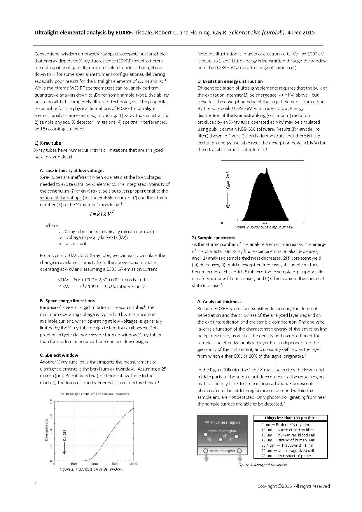
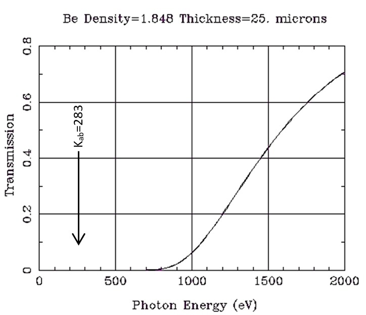
Figure 1. Transmission of Be window.
Figure 2. X-ray tube output at 4kV.
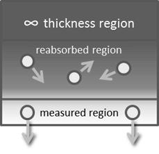
Figure 3. Analyzed thickness.
Things less than 100 μm thick
_________________________
4 μm — Prolene® X-ray film
10 μm — width of cotton fiber
10 μm — human red blood cell
17 μm — strand of human hair
25.4 μm — 1/1000-inch, 1 mil
50 μm — an average-sized cell
70 μm — thin sheet of paper
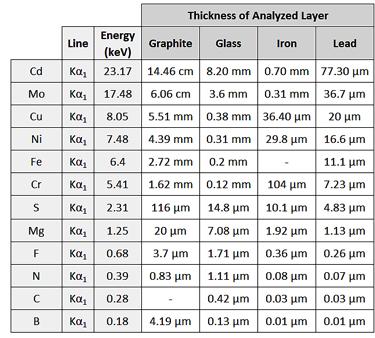
Table 1. Thickness of analyzed layer.
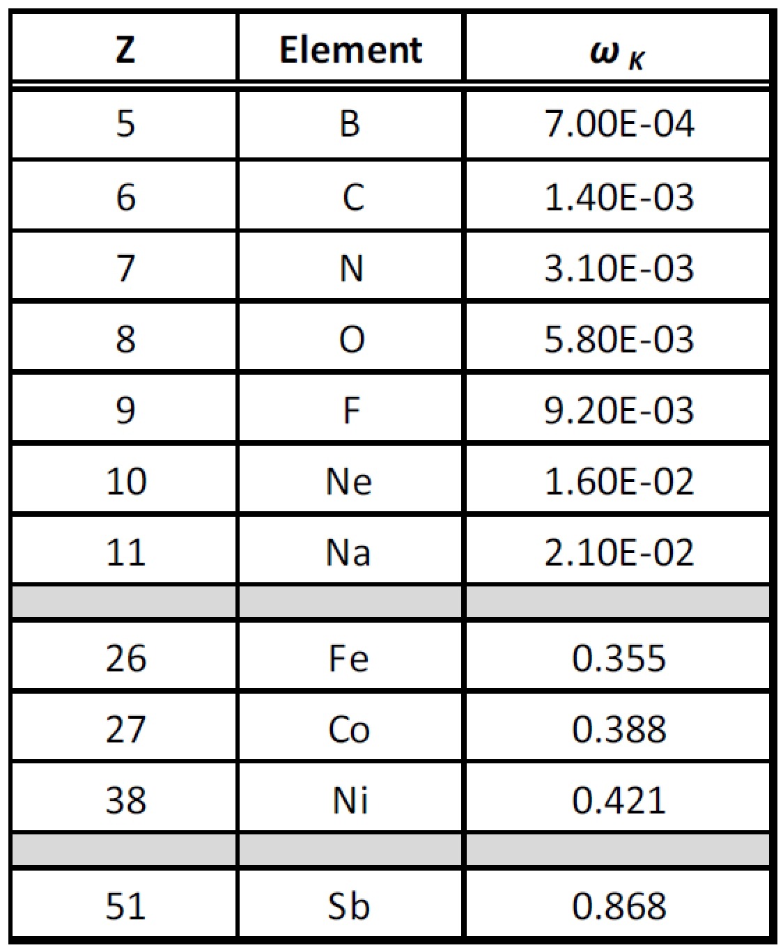
Table 2. Fluorescent yields.
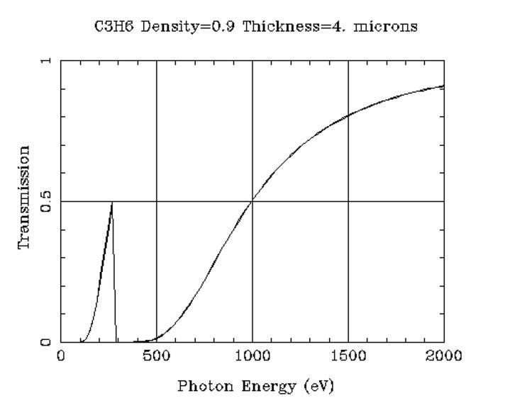
Figure 4. Transmission of Prolene window.
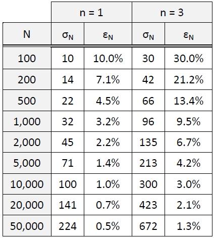
Table 3. Counting statistics.
About the Authors
*Robert C. Tisdale (drtisdale@gmail.com) received his Ph.D. in inorganic chemistry from the University of Nebraska – Lincoln in 1986 and M.B.A. in technology management from The University of Texas at Austin in 1988. Dr. Tisdale lives in Austin, Texas and has worked in the analytical chemistry field for over 40 years. He specializes in the strategic management and analytical marketing of scientific equipment and related technologies.
Ray R. Fleming received his Bachelors of Science degree from the University of Houston in 1986. Mr. Fleming lives in Austin, Texas and has worked in the field of health physics for 27 years. He is currently the Manager of the Radioactive Material Licensing Group of the Texas Department of State Health Services.